Datasets:
The dataset viewer is not available because its heuristics could not detect any supported data files. You can try uploading some data files, or configuring the data files location manually.
This Dataset is part of The Well Collection.
How To Load from HuggingFace Hub
- Be sure to have
the_wellinstalled (pip install the_well) - Use the
WellDataModuleto retrieve data as follows:
from the_well.benchmark.data import WellDataModule

# The following line may take a couple of minutes to instantiate the datamodule
datamodule = WellDataModule(
    "hf://datasets/polymathic-ai/",
    "viscoelastic_instability",
)
train_dataloader = datamodule.train_dataloader()

for batch in dataloader:
    # Process training batch
    ...
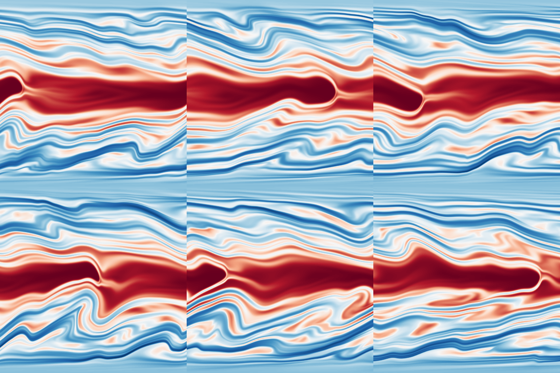
Multistability of viscoelastic fluids in a 2D channel flow
One line description of the data: Multistability in viscoelastic flows, i.e. four different attractors (statistically stable states) are observed for the same set of parameters depending on the initial conditions.
Longer description of the data: Elasto-inertial turbulence (EIT) is a recently discovered two-dimensional chaotic flow state observed in dilute polymer solutions. Two-dimensional direct numerical simulations show (up to) four coexistent attractors: the laminar state (LAM), a steady arrowhead regime (SAR), Elasto-inertial turbulence (EIT) and a ‘chaotic arrowhead regime’ (CAR). The SAR is stable for all parameters considered here, while the final pair of (chaotic) flow states are visually very similar and can be distinguished only by the presence of a weak polymer arrowhead structure in the CAR regime. Both chaotic regimes are maintained by an identical near-wall mechanism and the weak arrowhead does not play a role. The data set includes snapshots on the four attractors as well as two edge states. An edge state is an unstable state that exists on the boundary between two basins of attractors, the so-called edge manifold. Edge states have a single unstable direction out of the manifold and are relevant since the lie exactly on the boundary separating qualitatively different behaviours of the flow. The edge states in the present data set are obtained through edge tracking between the laminar state and EIT and between EIT and SAR.
Associated paper: Paper.
Domain experts: Miguel Beneitez and Richard Kerswell, DAMTP, University of Cambridge, UK.
Code or software used to generate the data: Dedalus.
Equation:
where is the streamwise and wall-normal velocity components, is the pressure, is the positive definite conformation tensor which represents the ensemble average of the produce of the end-to-end vector of the polymer molecules. In 2D, 4 components of the tensor are solved: . is the polymer stress tensor given by the FENE-P model.
| Dataset | FNO | TFNO | Unet | CNextU-net |
|---|---|---|---|---|
viscoelastic_instability |
0.7212 | 0.7102 | 0.4185 |
Table: VRMSE metrics on test sets (lower is better). Best results are shown in bold. VRMSE is scaled such that predicting the mean value of the target field results in a score of 1.
About the data
Dimension of discretized data:
- EIT: 34 trajectories with 60 timesteps, 512x512 images (chaotic solution).
- CAR: 39 trajectories with 60 timesteps, 512x512 images (chaotic solution).
- SAR: 20 trajectories with 20 timesteps, 512x512 images (simple periodic solutions).
- Transition to chaos between EIT and SAR: 36 snapshots with 20 timesteps of 512x512 images.
- Transition to non-chaotic state between EIT and SAR: 38 snapshots with 20 timesteps of 512x512 images.
- Transition to chaos between EIT and Laminar: 43 snapshots with 20 timesteps of 512x512 images.
- Transition to non-chaotic state between EIT and Laminar: 49 snapshots with 20 timesteps of 512x512 images.
Fields available in the data: pressure (scalar field), velocity (vector field), positive conformation tensor ( are in tensor fields, in scalar fields).
Number of trajectories: 260 trajectories.
Estimated size of the ensemble of all simulations: 66 GB.
Grid type: uniform cartesian coordinates.
Initial conditions:
- Edge trajectory: linear interpolation between a chaotic and a non-chaotic state.
- SAR: continuation of the solution obtained through a linear instability at a different parameter set using time-stepping.
- EIT: laminar state + blowing and suction at the walls.
- CAR: SAR + blowing and suction at the walls.
Boundary conditions: no slip conditions for the velocity at the wall and at the wall for the equation for .
Simulation time-step: various in the different states, but typically .
Data are stored separated by (\(\Delta t\)): various at different states, but typically 1.
Total time range (\(t_{min}\) to ): depends on the simulation.
Spatial domain size (\(L_x\), , ): , .
Set of coefficients or non-dimensional parameters evaluated: Reynold number , Weissenberg number , , , .
Approximate time to generate the data: 3 months to generate all the data. It takes typically 1 day to generate snapshots.
Hardware used to generate the data: typically 32 or 64 cores.
What is interesting and challenging about the data:
What phenomena of physical interest are catpured in the data: The phenomena of interest in the data is: (i) chaotic dynamics in viscoelastic flows in EIT and CAR. Also note that they are separate states. (ii) multistability for the same set of parameters, the flow has four different behaviours depending on the initial conditions.
How to evaluate a new simulator operating in this space: A new simulator would need to capture EIT/CAR adequately for a physically relevant parameter range.
Please cite the associated paper if you use this data in your research:
@article{beneitez2024multistability,
  title={Multistability of elasto-inertial two-dimensional channel flow},
  author={Beneitez, Miguel and Page, Jacob and Dubief, Yves and Kerswell, Rich R},
  journal={Journal of Fluid Mechanics},
  volume={981},
  pages={A30},
  year={2024},
  publisher={Cambridge University Press}
}
- Downloads last month
- 129
